

Contents
Overview
Ridom Typer supports for Windows users with installed Windows Subsystem for Linux (WSL) and Linux users starting from Illumina raw reads the analysis of SARS-CoV-2 tiled amplicon (e.g., ARTIC, AmpliSeq, or EasySeq RC-PCR) data. BWA-MEM is used to map the FASTQ files to the seed-/reference-genome MN908947.3 (NC_045512). The iVar tool trims the primers from the BAM file with the help of a supplied BED file that contains the primer positions. Finally, Samtools mpileup and iVar generate a whole genome FASTA consensus sequence file and determine variants (including low frequency variants; see below).
Those genomic FASTA files can be analyzed by two task templates. The SARS-CoV-2 Pangolin task template determines from the genomic FASTA file a PANGO lineage (Phylogenetic Assignment of Named Global Outbreak Lineages; e.g., B.1.1.7). This task template requires an Internet connection as the FASTA file is uploaded for analysis to a pangolin server run by Ridom. This server does not store any result or sequence data and checks daily for pangoLEARN lineage assignment updates.
The SARS-CoV-2 all ORFs task template separates the genomic sequence into subsequences matching the different open reading frames (ORFs). Read level quality control (QC) can be performed for all ORFs and FASTA consensus sequences can be conveniently edited. In addition, the task template queries the spike protein ORF for notable missense mutations that have a known or presumed effect for transmissibility, virulence, or antigenicity (Wikipedia, as of 5th January, 2022).
In the current SARS-CoV-2 all ORFs task template (version 1.5), the following positions of notable/shared mutations are defined in the S gene:
| Noteable Missense Mutation | Example(s)* | Gene | Start Genome Position |
Start Gene Position |
AA Number | Ref NT | Mutation NT | Ref AA | Mutation AA |
|---|---|---|---|---|---|---|---|---|---|
| S:HV69-70del | Omicron (BA.1, BA.3), Alpha, Eta (B.1.525), Cluster 5 | S | 21765 | 203 | 69-70 | TACATG | ------ | HV | -- |
| S:RSYLTPGD246-253N | Lambda (C.37) | S | 21987 | 425 | 246-253 | GTGTTTATT | --------- | SVYY | D |
| S:N440K | Omicron (BA.1, BA.2, BA.3) | S | 22880 | 1318 | 440 | AAT | AAG/AAA | N | K |
| S:L452R | Delta, Epsilon (B.1.429, B.1.427), Kappa (B.1.617.1) | S | 22916 | 1354 | 452 | CTG | CGG/CGT/CGC/CGA/AGA/AGG | L | R |
| S:Y453F | Cluster 5 | S | 22919 | 1357 | 453 | TAT | TTT/TTC | Y | F |
| S:S477G | S | 22991 | 1429 | 477 | AGC | GGT/GGC/GGA/GGG | S | G | |
| S:S477N | Omicron (BA.1, BA.2, BA.3), B.1.620 | S | 22991 | 1429 | 477 | AGC | AAC/AAT | S | N |
| S:E484K | Alpha (B.1.1.7 with E484K), Beta, Eta (B.1.525), Iota (B.1.526), B.1.620, Gamma, Zeta (P.2), Theta (P.3) | S | 23012 | 1450 | 484 | GAA | AAA/AAG | E | K |
| S:E484Q | Kappa (B.1.617.1) | S | 23012 | 1450 | 484 | GAA | CAA/CAG | E | Q |
| S:F490S | Lambda (C.37) | S | 23030 | 1468 | 490 | TTT | AGT/TCT/AGC/TCG/TCC/TCA | F | S |
| S:N501Y | Omicron (BA.1, BA.2, BA.3), Alpha, Beta, Gamma, Theta (P.3) | S | 23063 | 1501 | 501 | AAT | TAT/TAC | N | Y |
| S:N501S | Delta variant | S | 23063 | 1501 | 501 | AAT | AGT/TCT/AGC/TCG/TCC/TCA | N | S |
| S:D614G | Omicron (BA.1, BA.2, BA.3), Delta, Alpha, Beta, Epsilon (B.1.427, B.1.429), Eta (B.1.525), Iota (B.1.526), Kappa (B.1.617.1), B.1.620, Gamma, Zeta (P.2) | S | 23402 | 1840 | 614 | GAT | GGT/GGC/GGA/GGG | D | G |
| S:Q677P | bird mutations (e.g., Pelican, Robin 1) | S | 23591 | 2029 | 677 | CAG | CCT/CCG/CCC/CCA | Q | P |
| S:Q677H | bird mutations (e.g., Robin 2) | S | 23591 | 2029 | 677 | CAG | CAT/CAC | Q | H |
| S:P681H | Omicron (BA.1, BA.2, BA.3), Delta, Alpha, Kappa (B.1.617.1), B.1.1.207, B.1.620 | S | 23603 | 2041 | 681 | CCT | CAT/CAC | P | H |
| S:P681R | Delta, Kappa (B.1.617.1) | S | 23603 | 2041 | 681 | CCT | CGT/CGC/CGA/CGG | P | R |
| S:A701V | Beta, Iota (B.1.526) | S | 23663 | 2101 | 701 | GCA | GTT/GTG/GTC/GTA | A | V |
- with Alpha = B.1.1.7, Beta = B.1.351, Gamma = P.1/B.1.1.28.1, Delta = B.1.617.2, and Omicron = B.1.1.529 (BA.1 = B.1.1.529.1, BA.2 = B.1.1.529.2, and BA.3 = B.1.1.529.3).
Sequences and metadata can be batch-uploaded and imported from GISAID. Furthermore, a multiple FASTA export is implemented for visualization of those data with Nextstrain.
Consensus FASTA sequence files from Illumina, other sequencing platforms, or non-tiled amplicon approaches (e.g., metagenomic) can be analyzed by all Windows users. By automatically using the SARS-CoV-2 database scheme the database fields are compliant with the GISAID SARS-CoV-2 standards and the ENA virus pathogen reporting standard checklist. Due to rather few targets and quite frequently missing alleles it is recommend doing phylogenetic analysis in a comparison table from SNP rather than from allele haplotypes.
Step by Step Instruction
Installation
The iVar software must be available on the computers where the Ridom Typer Clients are installed, that perform the pipeline for processing Illumina tiled amplicon raw read data:
- Windows users must perform the Windows Subsystem For Linux (WSL) Installation.
- Linux users must perform the Installation of Bioinformatic Tools for Linux OS.
Processing and Analyzing
- Step 4: Create a new project, press the button Download & Add, select in the drop-down box at the top of the window Virus, download the two task templates SARS-CoV-2 Pangolin and SARS-CoV-2 all ORFs, and save the project by pushing the OK button.
 Hint: New Ridom Typer users find more details on how to setup a project and pipeline script in the Tutorial for Ridom Typer Assembly and cgMLST Analysis Pipeline.
- Step 5: Create a new pipeline script.
- Step 6: In the panel Define Input Sources of the script choose the FASTQs (e.g., the evaluation data below) and select as Procedure Details "Amplicon, viral RNA, Illumina, paired-end reads" or create own procedure details. If a submission to GISAID make a copy of the "Amplicon, viral RNA, Illumina, paired-end reads" Procedure Details and add at least the used Sequencing Platform.
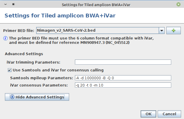
- Step 7: In the panel Define Projects choose the project and choose as assembler Tiled amplicon BWA+iVar (reference mapping). Press the Settings... button right of the assembler box. A primer BED file must be selected here. Primer BED files for ARTIC v3, Illumina AmpliSeq, NimaGen EasySeq RC-PCR v3, and Qiagen QIAseq SARS-CoV-2 Primer Panel and QIASeq DIRECT SARS-CoV-2 are provided. Either select one of the provided files or add via the + button a BED file with the primer positions for another protocol. Below the BED file dialog, the Advanced Settings... can be used to change iVar and Samtools mpileup command line parameters. For primer trimming Ridom Typer applies by default the -e option of iVar trim, i.e., reads with no primers will not be excluded from further analysis (e.g., ARTIC, Illumina AmpliSeq, or Qiagen QIAseq SARS-CoV-2 Primer Panel). Only in case that the amplicons are not fragmented during library preparation this option should not be used (e.g., NimaGen EasySeq RC-PCR, or Qiagen QIASeq DIRECT SARS-CoV-2). For provided BED files the -e option is set automatically correct. For Samtools mpileup mostly default parameters are used. The only non-default parameters used are do not discard anomalous read pairs (-A), disable per-base alignment quality (-B), skip bases with base quality smaller than 0 (-Q 0), and especially the maximum per-file coverage -d 1000000. The coverage of the pool amplicons can vary more than 100x in tiled amplicon approaches. Therefore, the value of the -d parameter should be at least 5-10x greater than the Avg. Coverage (Unassembled). For consensus calling by default the minimum quality score threshold (-q 20), minimum coverage to call consensus (-m 10), and minimum frequency threshold (-t 0.7) parameter values are applied. For stricter consensus calling, e.g., a called base must make up at least 90% presence at a position, the latter parameter must be changed to -t 0.9. For further details and other parameters it is referred to the iVar manual. All by Ridom Typer employed iVar and Samtools mpileup parameters are logged and can be found in the Assembly Post-processing row of the samples Procedure tab.
When pressing Next in the Define Project panel, the Mash Screen contamination check will be disabled in this pipeline even when it was select at the begin of the script definition as such a check is not required for species-specific tiled amplicon approaches. Furthermore, if previously no BED file was select a dialog for choosing such a file opens.
- Step 8: In the panel Define Submission leave the default setting Automatically assign local allele types to new alleles - it is impossible to submit new alleles to cgMLST.org as this is not foreseen for the SARS-CoV-2 task templates - and press Next.
- Step 9: In the panel Define File Management select the Assembly Result Files option Copy aligned read files to folder and select a folder, if later read level QC must be done (see below). If it is intended to submit sequence data to a repository such as GISAID, keep those BAM files at least until the data were accepted by the repository. Save the script and start the script.
- Step 10: After the pipeline has finished processing the data, exit the pipeline mode, and open the samples in the interactive mode. The samples Results tab will show the Pangolin lineage, Scorpio call, and the found notable/shared mutations. For more details open on the left in the navigation pane the task templates (e.g., QC support or Scorpio support).
- Step 11: When creating a comparison table for a project with the two task templates, it will contain as task result fields the Pangolin lineage (used for coloring by default), the Noteable Mutations, and the allele types for the 11 ORFs. For phylogenetic comparisons it is recommend to use the command Tools | Find SNVs in Distance Columns.... In the finally upcoming SNV Positions table push the Open in Variant Comparison Table icon. Once the comparison table has opened push either the Minimum Spanning Tree or Neighbor Joining Tree icon for tree drawing. The 11 ORFs cover 97.9% of the SARS-CoV-2 genome. Just short non-coding stretches - that are anyway usually not complete sequenced - at the begin and end of the genome are not covered.
Quality Control
Overview
The samples Procedure tab summarizes all available quality criteria. As an important pre-analytical criterion samples with a Ct value above 30 should be excluded from sequencing. The Perc. Covered Genome should be above 97.5% and the number of Ns should be below 1,000. Furthermore the Avg. Coverage (Assembled) should exceed 1,000. Finally, the number of Low Frequency Variants (frequency <70%) should not exceed 10 at maximum. An elevated value might indicate in falling order of probability a too high Ct, sample cross contamination, or co-infection with two strains. A genome-wide list with all variants (including low frequency variants) can be found attached down in the Procedure tab. If IGV (see below) is installed a coverage plot (e.g., for checking of 'pool failure') can be viewed by clicking the Show Coverage Plot in IGV link (it may happen that IGV does not show initially the coverage plot correctly; in this case elicit the IGV command File | Reload Tracks). Targets are colored red in the navigation pane if they contain frameshifts or are truncated. Yellow colored targets either contain ambiguities (Ns) or do not have a start and/or stop codon or contain an internal stop codon. Finally, all called ORFs variants to the reference genome can be viewed in a list when the button Show all Target Variants of the SARS-CoV-2 all ORFs Task is pushed. In the upcoming window with a list of all target variants is for each variant among others the variant read frequency (Var. Read Freq.) and the read coverage (Total Coverage) at the variant position stated. Selecting and clicking a row/variant of the list immediately opens the Contig Sequence Editor of the target and the position of the variant.
Variant Calling
To take a deeper look into the variants, iVar is also run for a variant calling. By default, iVar variant calling is run with the parameters -q 20 -m 10 -t 0.1
(see iVar manual]).
The result of the variant calling is stored as tsv file, and can be shown in the Procedure tab by clicking on the file link Variants.tsv.gz. It contains the following 19 columns:
| REGION | Region from BAM file |
| POS | Position on reference sequence |
| REF | Reference base |
| ALT | Alternate Base |
| REF_DP | Ungapped depth of reference base |
| REF_RV | Ungapped depth of reference base on reverse reads |
| REF_QUAL | Mean quality of reference base |
| ALT_DP | Ungapped depth of alternate base. |
| ALT_RV | Ungapped deapth of alternate base on reverse reads |
| ALT_QUAL | Mean quality of alternate base |
| ALT_FREQ | Frequency of alternate base |
| TOTAL_DP | Total depth at position |
| PVAL | p-value of fisher's exact test |
| PASS | Result of p-value <= 0.05 |
| GFF_FEATURE | ID of the GFF feature used for the translation |
| REF_CODON | Codong using the reference base |
| REF_AA | Amino acid translated from reference codon |
| ALT_CODON | Codon using the alternate base |
| ALT_AA | Amino acid translated from the alternate codon |
Read Level QC with IGV
If there should arise the need for a quality control on read level (e.g., truncation of a gene, internal stop codon, and/or frameshift) and the BAM files were kept (step 9 above) then the reads can be inspected with the Broad's Integrative Genomics Viewer (IGV). If IGV (with included Java) was installed in the default location, Ridom Typer can even hand-over the genome position. In the Contig Sequence Editor of a sample select a position in the target sequence and push the ![]() IGV button in the Ref.-seq. Align Panel. For IGV to work quicker the tool must be started once beforehand, in the upper left box More ... must be chosen, in the upcoming Genomes to add to list dialog SARS-CoV-2 must be filtered with the option Download Sequence checked, the OK button must be pushed, and IGV must be closed. If at another position the reads of the same sample must be controlled, pushing the IGV button will open a second instance of the viewer. However, the reads can quicker be inspected in the IGV Viewer if the position is selected in the Contig Panel of Ridom Typer, the base is right-clicked and from the context menu the command Copy current abs. position to clipboard is chosen. Next paste the clipboard content into the second box on top of the IGV viewer (keep the chromosome notation, i.e., enter the position after the colon) and press Return. If IGV was not installed in the default location or Ridom Typer cannot find for whatever reason the path to IGV, then the path to the installation folder can be entered once manually via the Options | Preferences | External Applications | IGV Path command.
IGV button in the Ref.-seq. Align Panel. For IGV to work quicker the tool must be started once beforehand, in the upper left box More ... must be chosen, in the upcoming Genomes to add to list dialog SARS-CoV-2 must be filtered with the option Download Sequence checked, the OK button must be pushed, and IGV must be closed. If at another position the reads of the same sample must be controlled, pushing the IGV button will open a second instance of the viewer. However, the reads can quicker be inspected in the IGV Viewer if the position is selected in the Contig Panel of Ridom Typer, the base is right-clicked and from the context menu the command Copy current abs. position to clipboard is chosen. Next paste the clipboard content into the second box on top of the IGV viewer (keep the chromosome notation, i.e., enter the position after the colon) and press Return. If IGV was not installed in the default location or Ridom Typer cannot find for whatever reason the path to IGV, then the path to the installation folder can be entered once manually via the Options | Preferences | External Applications | IGV Path command.
Editing Sample Contig File (FASTA)
If sequence edits are required then those edits should be stored also in the Sample Contig File (FASTA) as this is the only sequence file that is submitted to GISAID. Therefore, once one or more bases have been edited in the Contig Sequence Editor of a target there becomes the ![]() button active in the Contig Panel for storing those edits in the Sample Contig File. Please note that those edits need to be stored for each target separately as they are otherwise lost (a warning will be shown after editing a target and switching to another target without storing).
button active in the Contig Panel for storing those edits in the Sample Contig File. Please note that those edits need to be stored for each target separately as they are otherwise lost (a warning will be shown after editing a target and switching to another target without storing).
GISAID
To review the nucleotide insertions or deletions in sequences before submitting to GISAID optionally the GISAID online tool CoVsurver mutation app can be used. Own FASTA sequences can be submitted here and the reference sequence (WIV04) should be selected. Once the analysis is finished information about the non-synonymous changes per sequence is shown in a graphical manner. At the bottom of the website two links can be found. Those links allow to download additional data such as %N, nucleotide insertions and deletions, frameshifts, etc.
Export For GISAID
- Step 1: Invoke menu function File | Export Samples to GISAID Submission Files.
- Step 2: In the upcoming dialog select the to be exported samples and press OK.
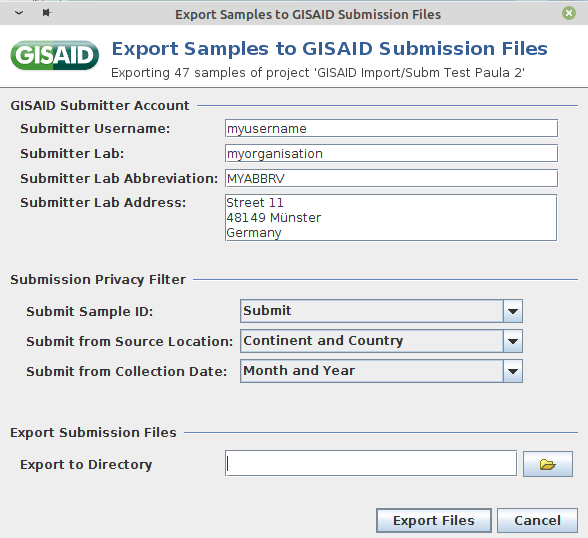
- Step 3: Enter username, lab, lab abbreviation, and lab address of your GISAID user account (those information will be remembered for the following submission).
- Step 4: Use the settings in Submission Privacy Filter to replace Sample ID with Alias ID and to specify the detail level for location and collection data.
- Step 5: Define at the bottom the directory where the two submission files should be saved. Then confirm the dialog with the button Export Files.
- Step 6: If no error occurs, the files are saved and a dialog is shown that allows to open the CSV file with the metadata for checking the data. The table view can also be used to edit the values and overwrite the originally exported file when the Export Table button is pushed. However, please note that those edits are not stored back in the Ridom Typer database. If required field data are missing a dialog opens that lists all missing data. The list can be copied to the clipboard or saved in a file. To proceed all those missing data must be first entered in the database and then exported again (For entering data in the Authors database field right-click to see and select previous authors entries).
- Step 7: Once logged-in to GISAID at www.gisaid.org the two files can be uploaded via the Batch Upload form. Alternatively the Automated Uploading via CLI is also possible once a user gets approved for this approach.
Import of EPI_ISL_yxz Numbers
- Step 8: Once the uploaded data have been approved by a curator the user will receive an email with all assigned EPI_ISL_yxz numbers. To import those numbers in the Ridom Typer database the following procedure is recommended.
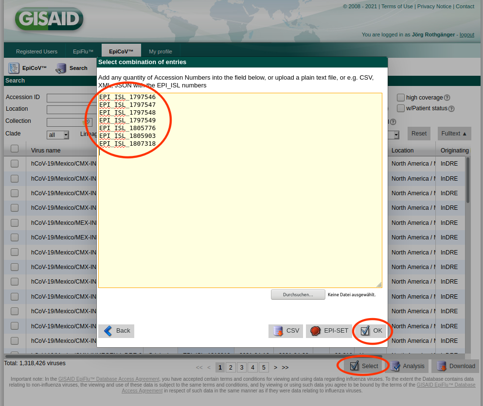
- Step 9: Copy the EPI_ISL_yxz numbers into the clipboard, log-in to GISAID, open Downloads, and push the Select button. Paste from the clipboard in the upcoming form the EPI_ISL_yxz numbers, press the OK button, and next press the Download button. Next select in the upcoming dialog the option Patient status metadata and save the file by pushing the Download button of this dialog.
- Step 10: In Ridom Typer elicit the menu function File | Open File(s), select the just downloaded Patient status metadata file, and press the Open button. In the upcoming Open Files dialog press the GISAID button, and select in the next upcoming Choose Project dialog the project that contains the to GISAID submitted samples and press the OK button. The finally upcoming Assigning GISAID Accession IDs window lists the samples with matching Sample or Alias IDs. If the matching was successful the EPI_ISL_yxz numbers were saved to the Nucleotide Accession(s) field of the Epi Characteristic section of the database scheme. Optionally the matching samples can be loaded in the Navigation Tree.
Import From GISAID
As the import of the more than one million GISAID SARS-CoV-2 entries into Ridom Typer is not feasible due to time constraints (would take several weeks), only the import of a selection of those entries is supported by Ridom Typer.
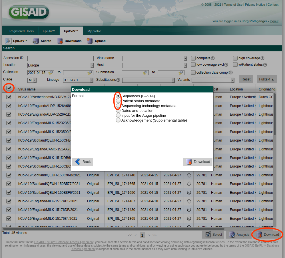
- Step 1: Log-in to GISAID, open Search, enter the search criteria of interest, select the those filtered entries by checking the checkbox in the column header, and push the Download button. Please note only 10,000 entries at once can be downloaded via this mechanism. In the upcoming Download dialog download the Sequences (FASTA) file by pushing the Download button. Push the Download button again, select this time the Patient status metadata file, and download the file. Once done, push the Download button again, select this time the Sequencing technology metadata file, and download this file too. The three just downloaded files must not be renamed and moved to a separate directory.
- Step 2: To import the data from the just downloaded three files elicit the menu function File | Open File(s), select the Sequences (FASTA) file, and press the Open button. In the upcoming Open Files dialog press the GISAID button, and select in the next upcoming Choose Project dialog the project in that the data should be imported. The EPI_ISL_yxz number will be used as Sample ID and the FASTA header (virus name) will be stored as Alias ID. Once the import process is finished a Imported from GISAID Download dialog opens that optionally allows to load the just imported samples in the Navigation Tree.
Nextstrain
For visualization of own data in a global phylogenetic context the sequence analysis webapp Nextclade of Nextstrain can be used.
- Step 1: In Ridom Typer invoke the menu function File | Export Sample Contig/SPEC Files ... . In the upcoming dialog select on top the to be exported samples. Furthermore, in the General Options dialog section choose for Export for selected samples the multiple fasta file containing all samples option. Press the OK button and choose the directory where to save the multiple fasta file.
- Step 2: Open Nextclade in a browser. Drag and drop the just exported multiple FASTA file in the Nextclade Sequences box. Next the analysis starts automatically. Once finished analysis results can be among others downloaded that include among others QC data, GISAID Clade, Nextstrain Clade, and/or the sequence data can be visualized in a tree.
Import of Genome-wide Consensus Assembly FASTA Files
Genome-wide consensus assembly FASTA files can be imported either via a pipeline (not using the assembly option) or via the Process Assembled Genome Data interactive option. Various genomes in a multiple-FASTA file cannot directly be processed (except those files from GISAID, see above). A multiple-FASTA file must be split into one FASTA file per sample/genome before it can be processed. Therefore, invoke the command Tools | Other Utilities | Split Multiple FASTA File into FASTA Files to perform such an operation before analyzing the resulting FASTA files.
Publication Ready Trees with Bootstrap
For producing publication ready trees with bootstrap support it is recommended to export from Ridom Typer the FASTA genome-wide consensus assembly files (invoke the menu function File | Export Sample Contig/SPEC Files ...). Next perform with those files a multiple alignment using MAFFT. From the multiple alignment file produce with IQ-TREE 2 a maximum likelihood tree. Finally, use a tool like FigTree to visualize the tree. Use similar or identical tool parameters as the authors of the PANGO lineage publication did. All three tools are free to use and all main operating systems are supported.
Evaluation Data
The example data archive Ridom_Typer_Examples_SARS-CoV-2_ARTICV3.zip (4.3 MB) can be downloaded for evaluation of the installation. Extract the zip-file on your computer. This evaluation data folder contains downsampled SRA Illumina paired-end FASTQ files of three SARS-CoV-2 samples. The data were produced using the ARTIC v3 tiled amplicon protocol. The PANGO lineage assignment should result in B.1.356, B.1.167, and B.1.1.7 for the three samples, respectively. Due to downsampling the coverage values are flagged in red.
FOR RESEARCH USE ONLY. NOT FOR USE IN CLINICAL DIAGNOSTIC PROCEDURES.