

Contents
Overview
This tutorial describes how to use the Ridom Typer software to assembly and analyze bacterial genomic data using the Ridom Typer Pipeline Mode.
Listeria monocytogenes is used exemplary for this demonstration. However, by reading this tutorial you should be able to define your own pipelines and projects for all species with a public available cgMLST scheme in the Task Template Sphere and analyze your own raw read data (FASTQ files) or preassembled data (FASTA files). If you intend to analyze in addition or exclusively public genomic data from either NCBI genomes or NCBI Sequence Read Archive (SRA) you can use Ridom Typer to download and process those data, too. Further details can be found on the pages Download from NCBI Genomes and Download FASTQ from SRA. If you are analyzing a species for which no public cgMLST is available yet, please take a look at Core Genome MLST Schemes help.
Like MLST, the genome-wide gene-by-gene allele calling cgMLST approach employed here, uses alleles as the unit of comparison, rather than nucleotide sequences. In allele-based comparisons among isolates, each allelic change is counted as a single genetic event, regardless of the number of nucleotide polymorphisms involved. This provides a simple and effective correction for the fact that in many bacteria, common horizontal genetic transfer events account for many more polymorphisms among specimens than rarer point mutations. The cgMLST approach retains information at all loci and avoids the need to categorize which changes are recent point mutations and which are due to recombination. As core and accessory genome MLST schemes record the sequences of allelic variants, those schemes can also be used for sequence-based analyses (e.g., SNP calling or using concatenated sequences) when this is appropriate (adapted from: Maiden MC, Jansen van Rensburg MJ, Bray JE, Earle SG, Ford SA, Jolley KA, McCarthy ND. MLST revisited: the gene-by-gene approach to bacterial genomics. Nature Rev Microbiol. 2013, 11: 728-36 [PubMed 23979428]).
Preliminaries
- Installation of Ridom Typer: If Ridom Typer is not available yet, a one-month trial version can be requested. The Ridom Typer Client and Server software can be installed on the same computer for this tutorial.
- System Requirements: This tutorial requires at least 8 GB RAM. It is recommended to use the tutorial on a Windows system with installed Windows Subsystem for Linux (WSL) or on a Linux system. With 8 GB RAM and Core i3 CPU the pipeline takes are around 20 minutes.
 Hint: If a Windows system without WSL is used for the tutorial, the Velvet Assembler must be used as an alternative de novo assembler for SKESA which increases the run time of the pipeline fourfold. Then 16 GB RAM are recommended and species identification, contamination check, NCBI AMRFinderPlus, and run details import are not available.
- Tutorial Data: Download the example data archive Ridom_Typer_Examples_Pipeline_L_monocytogenes_ACCO.zip (~270 MB) for this tutorial and extract the zip-file on your computer. This example data folder contains Illumina MiSeq 250bp paired-end FASTQ files for 4 isolates of Listeria monocytogenes. The FASTQ files were downsampled to 30x coverage to decrease the assembling time for this tutorial. The original whole genome shotgun (WGS) data was published by Ruppitsch et. al. (JCM 53: 2869–2876, 2015). To demonstrate the import of Illumina run details some artificial run info files were added to the example data folder.
Define Pipeline Script
- Step 1: Start the Ridom Typer Client without logging in and press the button
 Start Pipeline Mode on the bottom of the login panel or use the identical menu function in the File menu.
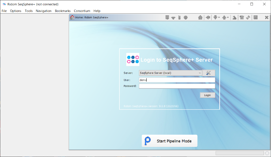
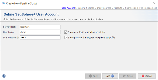
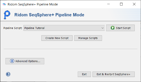
- Step 2: The pipeline mode window starts up. The pipeline mode is designed to run Ridom Typer in a non-interactive way to assemble, process, and analyze WGS data automatically defined by a pipeline script. Press Create New Script to open a dialog for creating a pipeline script. In the first step the Server Host and the User Login must be defined. Just use localhost for your local computer and the same Ridom Typer user account that you are normally using for the Ridom Typer login. The option to store user login in the pipeline script is enabled by default. Below enter the User Password of this user account. If wanted, the password can also be stored (encrypted) in the pipeline script. However, it should be taken into account that if the password is stored in the pipeline script, anyone with access to the computer can run the pipeline. For this tutorial check the Store password encrypted in pipeline script file checkbox.
- Press Next to move on.
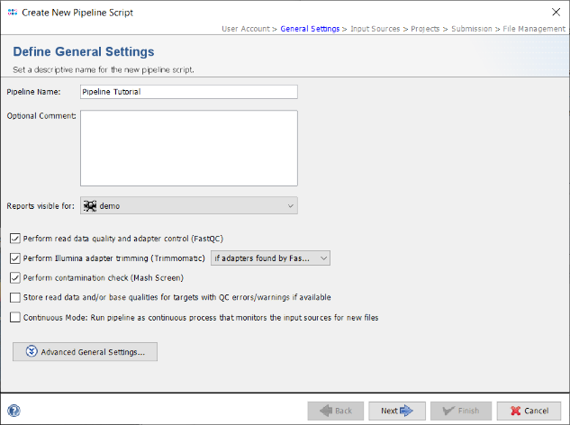
- Step 3: In the Define General Settings panel enter a Pipeline Name (e.g., 'Pipeline Tutorial'). The comment can be left empty and the access control for viewing the reports generated by this pipeline can be left to the user's group as default. If the Ridom Typer Client is running on Linux or on Windows with installed WSL five checkbox are shown. The first three checkboxes are preselected and allow to perform automatically a FASTQ file quality control with FastQC, an adapter trimming with Trimmomatic if adapters were found, and a contamination check with Mash. The fourth options allows to store read data in the database for problematic targets. The option "Continuous Mode" can be used to monitor a directory and automatically process newly appearing sequence data files. For this demonstration leave the latter two options unchecked.
- Press Next to move on.
- Step 4: In the next panel the Input Sources for the WGS sequence data are selected. The Input Source Type is predefined with Directory. Press the
 button and select the directory Ridom_Typer_Examples_Pipeline_L_monocytogenes_ACCO that was unpacked from the downloaded tutorial data file (see Preliminaries). The File Preview on the lower right shows the 8 fastq.gz files that are currently in this directory. When the pipeline is started all files in this directory will be processed. Files can be excluded from processing by selecting them via the right-click menu in the File Preview.
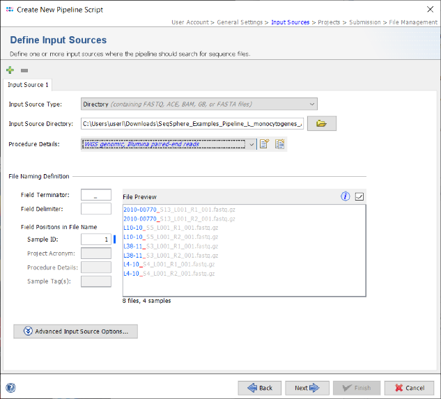
- Step 5: The Procedure Details must be selected for the sequence data files to document the laboratory procedure details for all Samples processed with this script. For this tutorial data select the predefined procedure details WGS genomic, Illumina, paired-end reads.
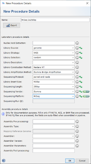
- Hint: Alternatively, for documentary purpose more details can be defined by pushing the
 New Procedure Details button. A New Procedure Details window pops-up. Enter at least Library Source: genomic, Library Strategy: WGS, Library Selection: random, Sequencing Protocol: paired-end reads, Library Insert Size: 400bp, Sequencing Length: 250bp, Sequencing Vendor: Illumina, and Sequencing Platform: MiSeq. Those details are required if later on a submission with Ridom Typer of the raw read data to the EBI European Nucleotide Archive (ENA; as also indicated by the green icons in the window) is intended (e.g., for publication purposes). The assembly procedure details can be left empty as they are filled-in when using the assembly pipeline. Press the OK button of the New Procedure Details window.
- Step 6: Each input source must also have a File Naming Definition that describes at least how to find the Sample ID in the file names of your sequence data. The Field Terminator is automatically filled with the underline (_) symbol. You can leave this to default for the tutorial data. If your own sequence file names do not fit this definition further details can be found in the file naming documentation. Press Next to move on.
- Step 7: In the next Define Projects panel the Project(s) are selected into which processed Sample data should be imported. For this tutorial the Project does not exist yet and must be created. If you don't have any projects at all in your database yet, a dialog will be shown automatically asking to create a procect. Confirm this dialog with OK. Else, press the button
 Manage Projects in Database in the bottom right of the window. In the upcoming Projects window, press the
  Create new Project icon to start defining a new project.
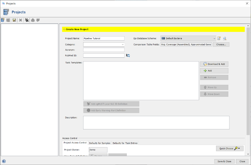
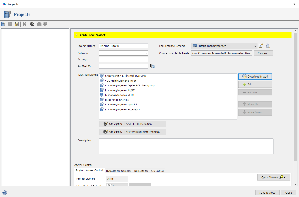
- Step 8: Enter a name for the new Project (e.g., Pipeline Tutorial). Then press
 Download & Add in Task Templates section to browse the Task Template Sphere.
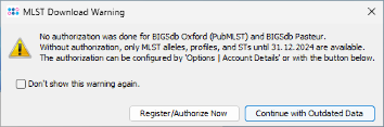
- Step 9: A MLST download warning dialog is shown. BIGSdb/pubMLST Oxford and Pasteur requires to have an account and an authorization to retrieve MLST alleles, STs, and schemes newer than 31 December 2024. For all tutorials such definitions are not needed. Therefore, just press Continue with Outdated Data to proceed. If you do not want to see this dialog again during following tutorials, mark the checkbox Don't show this warning again before clicking Continue. Once an account was registered at the pubMLST web site(s), the authorization can be activated in the Ridom Typer Account Details.
- Step 10: The Task Template Sphere provides all predefined public Task Templates. Choose as organism Listeria monocytogenes. There are eight Task Templates listed for L. monocytogenes, i.e., cgMLST, Accessory, MLST, 5-plex PCR Serogroup, NCBI AMRFinderPlus, Chromosome & Plasmids Overview, and CGE MobileElementFinder. The cgMLST Task Template defines the 1,701 genes of the reference strain EDG-e that are used for the public nomenclature and for the definition of the complex type (CT). The Accessory Task Templates defines in addition 1,158 genes that do not belong to the core genome. However, they can be used to increase the discriminatory power if the resolution of cgMLST is not high enough. The NCBI AMRFinderPlus task template is used to find antimicrobial resistance-specific proteins. The Chromosome & Plasmids Overview and the CGE MobileElementFinder task template are used to find plasmids and mobile elements.
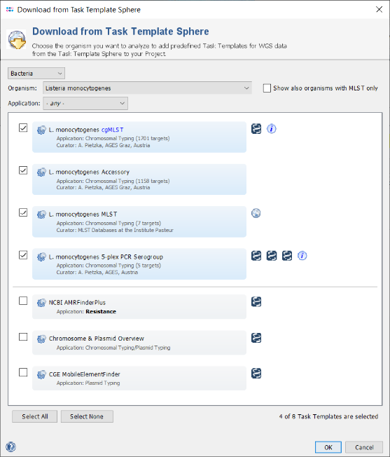
- Step 11: Select all Task Templates and press OK to download and to add them to the Project. Below the Task Templates panel, there two additional definitions can be added to the project: Firstly, Local Single Linkage Clustering IDs can be defined to assign SLC IDs automatically to the samples of the projects, according to their cgMLST profiles. This can be used to build a local cluster nomenclature. Secondly, Early Warning Alerts can be defined for the project. For this tutorial, we will define only an EWA. Therefore, press the button
 Add cgMLST Early Warning Alerts Definition.
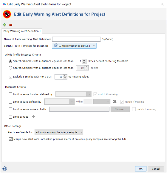
- Step 12: The upcoming window shows the definition of the first Early Warning Alert created for this project. All settings can be left to default, to define an alert that is triggered if two sample of the project have a distance of the cgMLST task templates default clustering threshold or below. Additionally, metadata criteria (e.g., place and time) can set here. For this tutorial, all should be left to defaults. Press the OK button of the Early Warning Alert window. Then finally press the Save & Close button in the Projects window, to close the window and store the newly defined project.
- Step 13: Now select the just created project in the Project Name field of the Define Projects panel.
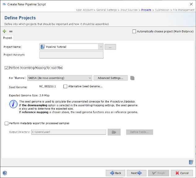
- Step 14: The seed genome for L. monocytogenes that is used as genome size reference for downsampling is automatically loaded from the cgMLST task template. Check the box Perform Assembling/Mapping for read files. If on Linux or Windows with installed WSL the de novo assembler SKESA is preselected and should be used for this tutorial else Velvet can be used for de novo assembling.
- Press Next to move on.
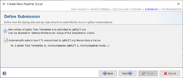
- Step 15: In the upcoming Define Submission panel can be defined if the pipeline should automatically submit the new alleles and the allelic profile to the public cgMLST Nomenclature Server (cgMLST.org). The submission of new alleles is enabled by default and can only be disabled globally in the Client. However, hereby the allelic profile of the Sample is not stored at cgMLST.org. If the option Automatically submit new CTs anonymized to cgMLST.org Nomenclature Server is checked, the allelic profile of the Sample with new CTs are stored on cgMLST.org anonymously without any epidemiological metadata. By default this checkbox is enabled in new pipeline scripts with the option.
- Press Next to move on.
- Step 16: Finally, in the Define File Management panel it can be defined what the pipeline should do with the created assembly files and raw reads. Leave all to default and press Test Pipeline Script to validate your pipeline.
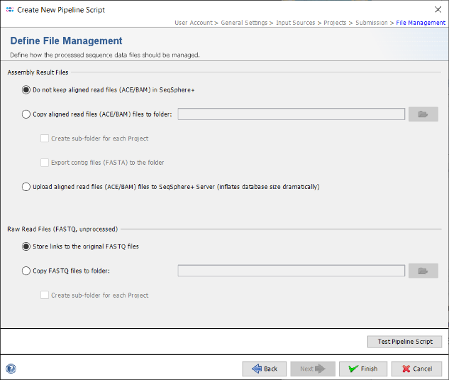
- Step 17: The test should finish successfully. Press the Close button of this dialog. Now press Finish to store the new pipeline script.
Run the Pipeline
- Step 1: Be sure that in the upcoming Pipeline Mode Window the just created pipeline script is selected and press the button
 Start Script to run the pipeline.
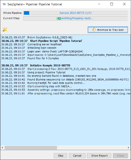
- Step 2: A blue colored progress window is opened showing the current progress and messages of the pipeline.
- If the SKESA de novo assembler is used, the pipeline will take about 20 minutes (8 GB RAM; Core i3 CPU) to finish. If Velvet is used the runtime is about quadrupled.
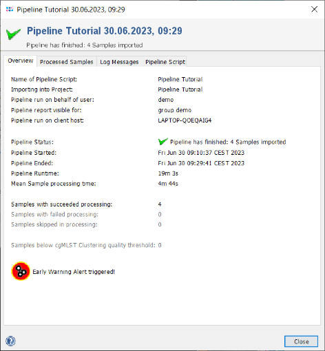
- Step 3: When the pipeline has finished the background color turns to white. Press the Show Report button to see a quick overview for the statistics of the processed Samples. The window contains the information that 4 samples were processed successfully, and it shows on the bottom an icon for a triggered early warning alert.
- Step 4: Close the report window, press Close in the pipeline progress window, and exit the pipeline mode with the button Exit and Restart Ridom Typer. Thereby it is switched back to the normal interactive session mode that allows for viewing the results of the just processed Samples.
- Hint: If you want to process additional files later in the same way and into the same project, you can just copy them into the file input directory that was chosen when creating the pipeline script. Then start the pipeline again to process the new files. Files that belong to samples that were already processed are automatically skipped.
Open the Processed Samples
- Step 1: The Ridom Typer Client login window appears again. Enter the user name and password and press Login to show the home screen.
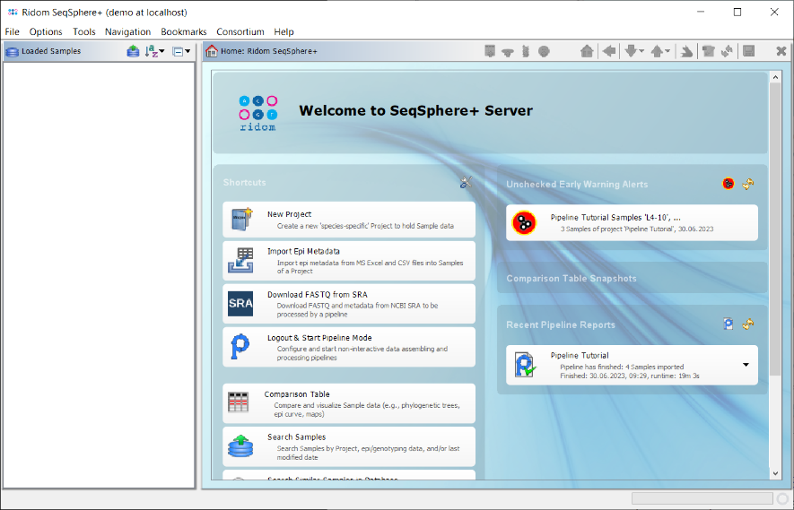
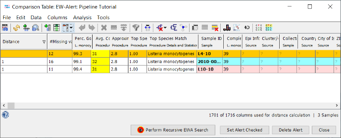
- Step 2: On the right of the home screen in the section Early Warning Alerts a red icon for a new alert is shown. Click it to open a comparison table containing the samples that triggered the alert. The table shows that three of the samples that were processed have an allelic distance below the predefined cgMLST clustering threshold, which could give a hint for an potential outbreak. To remove the Early Warning Alert from the home screen window, confirm the dialog with Set Alert Checked.
- Step 2: The Early Warning Alert is removed now. But in the section Recent Pipeline Reports an item for the new report is still shown. Click it to open the report or use the menu function
 Options | Browse Pipeline Reports to choose it from a list of all reports.
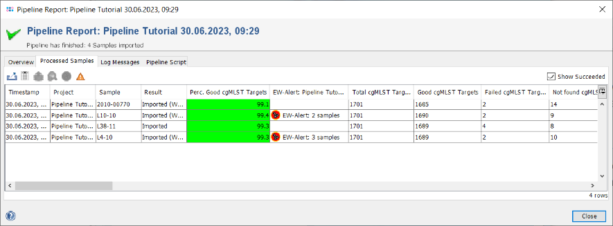
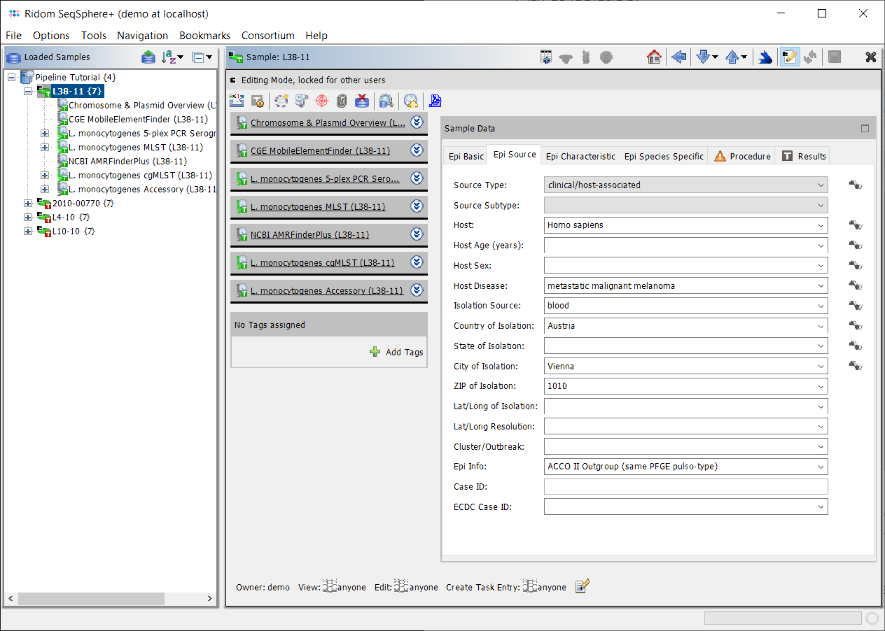
- Step 3: The pipeline report is the same as it was shown just before in the pipeline mode. As Ridom Typer is now in interactive mode Samples can be directly loaded into the workspace. Click the Processed Samples tab to show the four samples that were processed. The column Perc. Good cgMLST Targets is highlighted green, because all samples passed the defined QC threshold for it. Note the two Samples that are marked with the EW-Alert icon, because they triggered an alert when compared with the first sample, that was already stored in the database when they were processed. Double-click on the first Sample to load it in the background. Close the pipeline report window. The Sample is shown in the workspace.
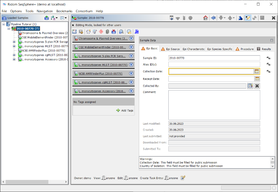
- Step 4: The left panel of the main window shows a navigation tree with the loaded Sample. Each Sample node in the navigation has six sub nodes: The 5-plex PCR Serogroup task, the MLST task, the AMRFinder task, the cgMLST task, and the Accessory task. Below the task nodes there are the target nodes. Each target node represents one sequence (here a gene) that was extracted from the input data (here the de novo assembled WGS data). The targets can have different target QC states (look here for more details about Target QC procedure parameters):
-
 Good Targets (green) were extracted and fulfilled all requirements that are defined in the Target QC Procedure of the Task Template.
-
 Good Targets with Warnings (yellow) were extracted and fulfilled all Target QC Procedure requirements that are relevant for errors, but failed the minimum coverage checks in Target QC Procedure.
-
 Failed Targets (red) were extracted but failed at least in one of the requirements that are defined in those parameters. For example, they may have frame shifts and incorrect lengths compared to the allele of the seed genome.
-
 Not Found Targets (gray) were not extracted (because the match did not reached the thresholds or the target is not present at all).
-
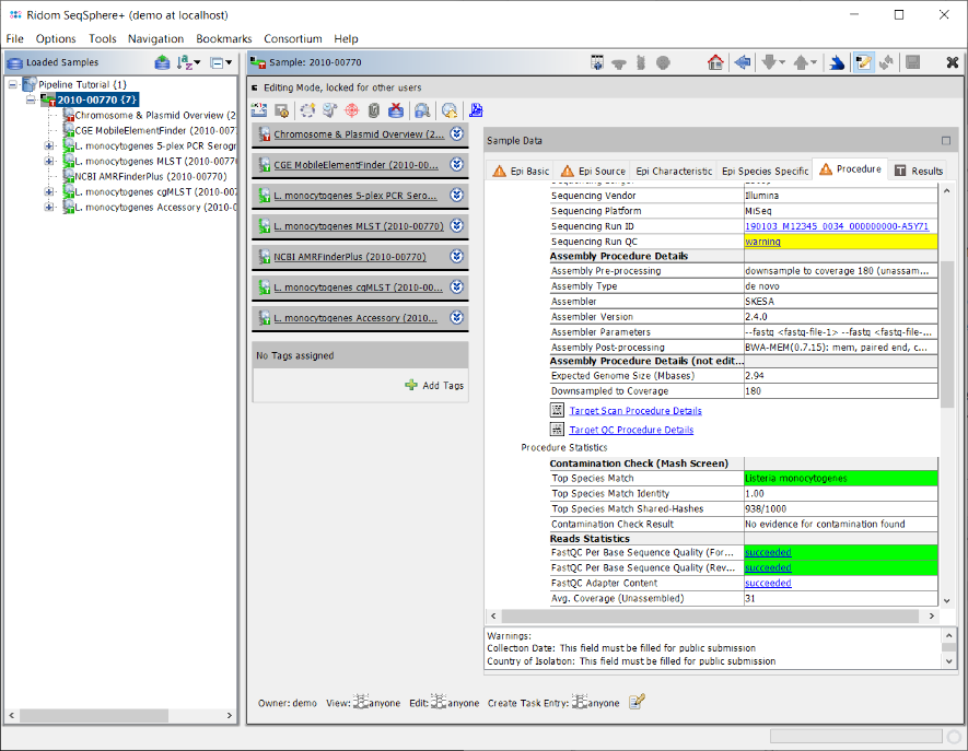
- Step 5: Click on the Procedure tab in the right panel of the window to see the details about the sequence data and processing. Some fields are important for quality control of the sequence data. Again traffic light colors are used to highlight their QC result status for various aspects as succeed, warning, or failed.
- In the Procedure Details section the values for Sequencing Run ID and/or Sequencing Run QC can be right-clicked to show the Sequencing Run Details if run info files were imported by the pipeline.
- In the Reads Statistics section the QC results of FastQC Per Base Sequencing Quality and FastQC Adapter Content can also be right-clicked to show the detailed FastQC results if FastQC was executed by the pipeline.
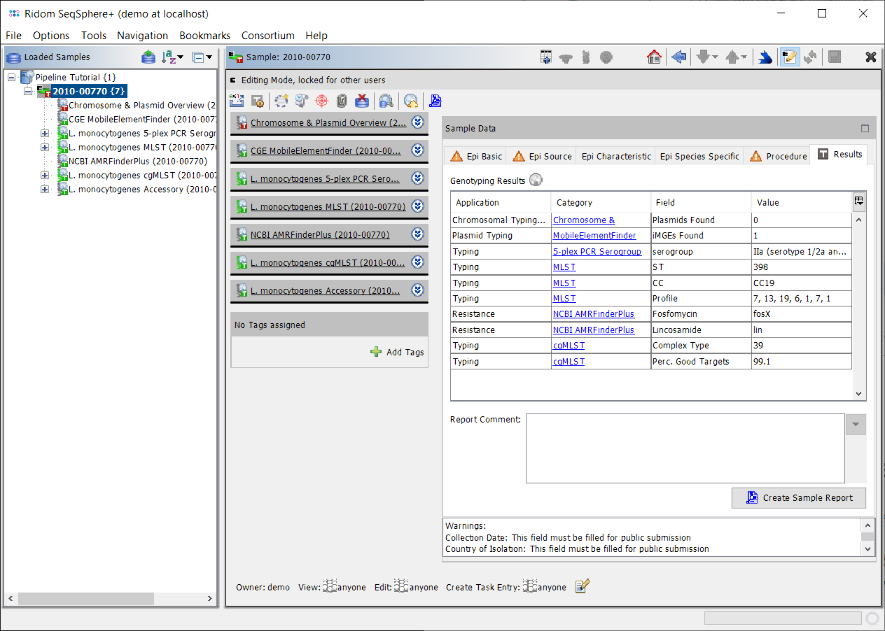
- Step 6: Click on the Results tab in the right panel of the window to see the Genotyping Results of the tasks that were processed for the sample. The result table has four columns: Application (e.g., Typing or Resistance), Category (corresponds with the task template name), Field (name of the specific result fields), and Value (the confident result value for this result field).
- The Category entries can be clicked to see the result details by browsing to the Task Entry Overview (e.g., to show the results of AMRFinderPlus).
- Step 7: Close the Sample by pressing the
 in the toolbar above the panel.
Import Epidemiological Metadata
- Step 1: Invoke in the menu File | Import Epi Metadata
- Step 2: In the upcoming Choose File to Import dialog select the file Lm_metadata.xls from the directory Ridom_Typer_Examples_Pipeline_L_monocytogenes_ACCO.

- Step 3: A preview dialog with the content of this Excel file is shown. It contains epidemiological metadata of the four Samples for which the sequence data was already processed. Press Continue.
- Step 4: The next dialog defines the import settings. First select on top the project that was created and processed by the pipeline before.
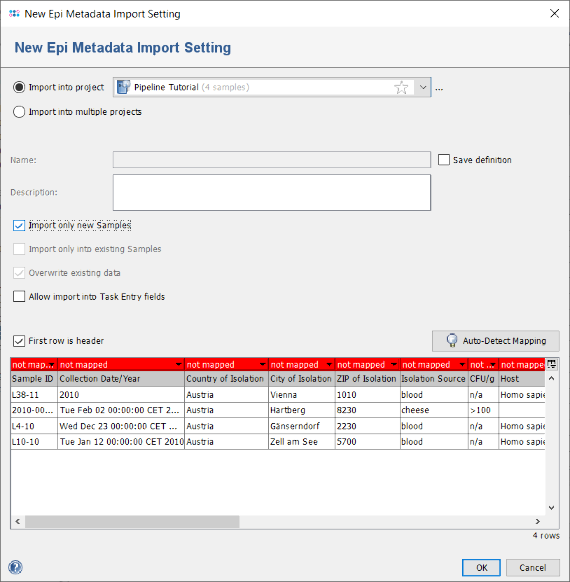
- Step 5: The table on the bottom shows the mapping between the table columns and the Ridom Typer database fields. By default all columns are unmapped and the headers are therefore highlighted in red. As the column headers have the same (or similar) name as the database fields, a mapping can be done automatically. Press the button Auto-Detect Mapping to recognize and map all known column names.
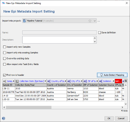
- Step 6: All but two columns were mapped to Ridom Typer database fields. For the two columns that are still with red headers (CFU/g and Outcome) no fields exist with that name in the Ridom Typer database. If they should be imported in the database they could be manually mapped to existing fields by clicking on the red header and selecting a field (those mappings can be stored for later re-usage for files with identical headings). If those fields does not exist, they must be created before invoking the metadata import. For this tutorial we leave the two fields unmapped. Press OK to start the import.
- Step 7: After the import is finished a dialog is shown. Press Open Samples to open the Samples and take a short look at the imported database fields (e.g., Collection Date and City of Isolation).
- Step 8: Close all Samples by choosing in the menu File | Close All.
Analyze Samples with Comparison Table and Draw a Tree and Epi Curve
- Step 1: Choose from the menu Tools | Comparison Table to draw a tree (phylogenetic analysis), an epi curve, and/or map.
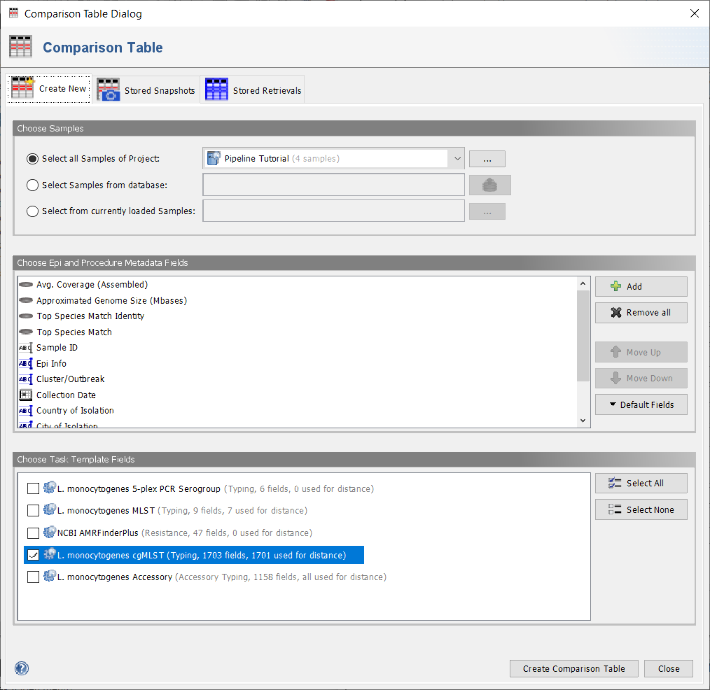
- Step 2: In the Comparison Table dialog go to the first tab "Create New". In the Choose Samples section choose the first option Select all Samples of Project and the new previously created project (e.g., Pipeline Tutorial). Below the default epidemiological and procedure metadata fields for the comparison table are listed. The button Default Fields can be used to store a different set of fields as default. On the bottom of the window the section Choose Task Template Fields shows checkboxes for all task templates of the selected project. By default only the checkbox for L. monocytogenes cgMLST is preselected, i.e. only the allele fields of this task template will be added to the comparison table. Use the default settings, press the Create Comparison Table button to confirm the dialog and create the comparison table. For details how to compare AMRFinder profiles it is referred to the documentation.
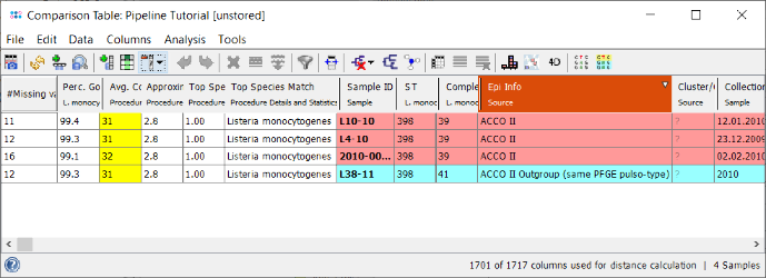
- Step 3: The comparison table is opened and shows the data for the four Samples. The column with the red header (Epi Info) is used by default for coloring the Sample rows. The columns with a dark green header are used for distance calculation. Those columns are the allele types of the cgMLST task. Some of those contain missing values if a cgMLST target was not found at all in an input sequence ("? (not found)") or if the Target QC Procedure for this target has failed, e.g., because of a frame shift error ("? (failed)"). The first column in the table shows the total number of missing distance values per row. The QC related field 'Avg. Coverage (Assembled)' is highlighted yellow as the coverage of the tutorial data is below 75 fold, but above 30 fold.
- Step 4: Right-click on the column Complex Type (ninth column) and choose from the menu
 Set Color Groups by Column Values. Leave the upcoming dialog to defaults and confirm with OK. The Sample rows are now colored by the different cgMLST CTs. Further description of functionality (e.g., sorting, filtering, and exporting of data) can be found in the Comparison Table documentation.
- Step 5: Press the
 Minimum Spanning Tree icon in the toolbar to calculate the distances between the Samples and draw a minimum spanning tree for them. Because the table contains missing data, it must first be confirmed that the missing values are ignored pairwise or another of the available options must be chosen. Just confirm the dialog with OK.
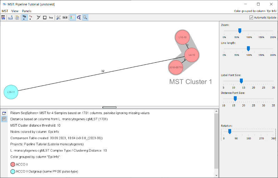
- Step 6: The minimum spanning tree is calculated for the allelic profiles of the 1,701 cgMLST targets (pairwise ignored missing values) and is shown in a new window. By default the nodes are again colored by the Complex Type (CT) and it can be easily seen that 3 of the 4 isolates have the same Complex Type (CT 39), as they all have a distance below 10 alleles to the CT founder. Just Sample L38-11 belongs to a different Complex Type.
- Two conclusions can be drawn from this tree.
- The three CT 39 isolates (with epi info ACCO II) have the same Complex Type and a close distance. The minimum spanning tree also found an MST cluster for the three isolates using the very same allelic distance threshold of 10 (labelled "MST Cluster 1"). Therefore, this MST cluster indicates epidemiological relationship.
- The fourth isolate (L38-11; with epi info ACCO II outgroup) has a different Complex Type and a distance of 32 alleles to the three other isolates and does not belong to the outbreak (in fact this isolate from the original publication was epidemically unrelated but shared with the three other isolates an identical pulsotype [by PFGE with two different enzymes]).
- Hint: The Minimum Spanning Tree (MST) can be exported by clicking the
 Export MST icon of the toolbar. In the upcoming Export MST file dialog choose as file type the Scalable Vector Graphics (*.svg) or Windows Enhanced Metafile (*.emf) format. Note that EMF or SVG are vector graphics formats and are therefore suited for finishing publication ready figures. EMF files can imported and scaled by MS PowerPoint. SVG files can be edited, e.g., with Adobe Illustrator or the open-source InkScape tool (once the file is loaded first ungroup all objects). Further description of MST functionality (e.g., cluster shading, figure legend, tree appearance, etc.) can be found in the Minimum Spanning Tree documentation.
- Step 7: Press the button
 to store the comparison table and the MST as Comparison Table Snapshot in the database for potential later reuse (accessible from the home screen in the section Comparison Table Snapshots).
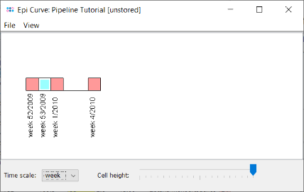
- Step 8: Press the button
 to create an Epi Curve from the comparison table data. As the collection dates were imported from the metadata file the Samples are shown in the graph ordered by date. The time scale of the epi curve can be changed. Samples with incomplete time data are shown with a white rectangle border (e.g., L38-10).
- Step 9: Press the button
 to create an Geographical Map from the comparison table data. The country and city information was imported from the metadata file but no latitude/longitude information exists yet. Therefore, a dialog is shown that offers to perform a geocoding (Internet connection is required for this functionality). Press the Do Geocoding button.
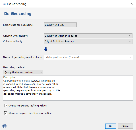
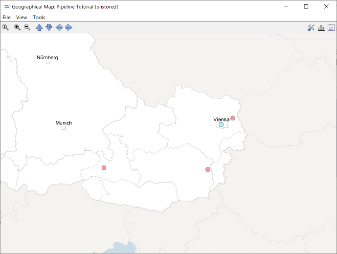
- Step 10: Leave the upcoming dialog to default settings and confirm it by pressing the OK button, to retrieve the geographical latitude and longitude for the city and country information that was imported as metadata. After this information was retrieved a dialog asks whether to store the latitude/longitude values in database. Go with the default setting by pressing the Yes, Store in Database button. Once done the window with the geographical map opens automatically. The four Samples are drawn on their geographical location. Clicking on a Sample in the map marks the Sample also in the epi curve, the minimum spanning tree, and in the comparison table (all those windows and the comparison table are interactively linked).
Find Group Specific SNVs for Screening Assay
- Step 1: The function
 Find Group Specific SNVs in the comparison table allows to find Single Nucleotide Variants (SNVs) that are unique to a group of Samples (target-genomes) and do not appear in a second group of Samples (nontarget-genomes). Those group specific SNVs can be used to develop highly specific screening assays (e.g., real-time PCR TaqMan™ or High-Resolution Melting Curve [HRMC] assays).
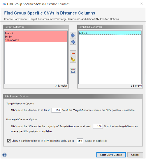
- Right-click on the column Epi Info and choose from the menu Set Color Groups by Column Values to set the coloring back to the epidemiological information. Now press the icon in the toolbar of the comparison table window to invoke the SNV search function. A dialog for the handling of missing values is shown, confirm it with the default settings. In the upcoming dialog choose the ACCO II isolates (with CT 39) as target-genomes and ACCO II Outgroup with L38-11 (CT 41) as nontarget-genome. Confirm the dialog by pressing the OK button.
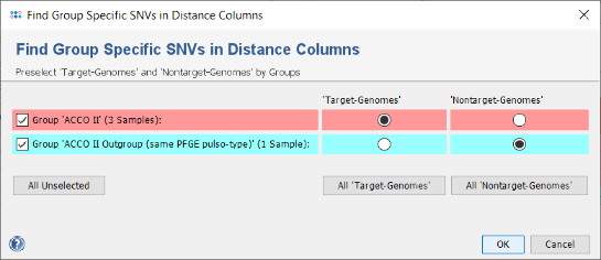
- Step 2: In the following dialog the Samples selection and some options are shown. If corrections are needed (or if no groups exist in the comparison table) the Samples can be removed or moved here between the target- and nontarget-genomes. The export button
 allows to write the FASTA files of all chosen Samples into two different directories (target-genomes and nontarget-genomes) to use them for a signature search with an external software (e.g., PanSeq Novel Region Finder). Such an export is not done in this tutorial.
- Confirm the dialog with default settings to start the search for group specific SNVs.
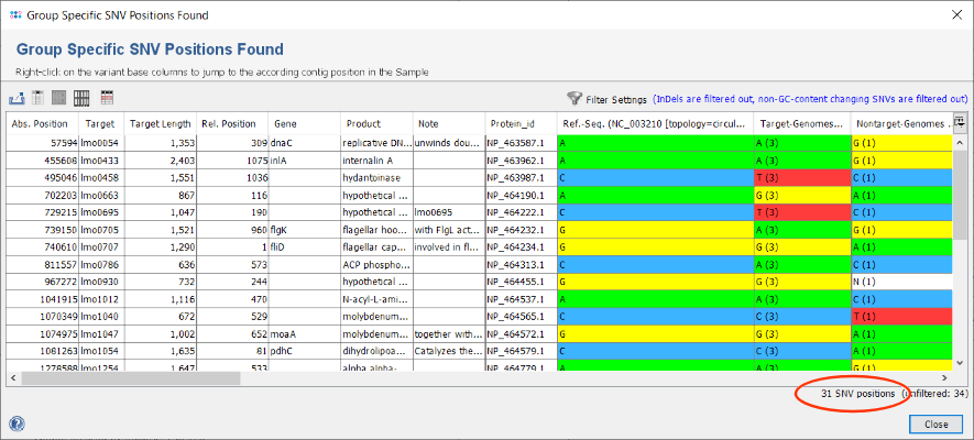
- Step 3: After the search has finished in total 34 SNVs were found. Each row of the table represents a group specific SNV that was found in all target-genomes but not in the nontarget-genomes. By default, the filter setting Show only substitution SNV positions is enabled. Therefore one InDel is filtered out and the table shows only 33 SNVs. The columns Target-Genomes and Nontarget-Genomes summarize the nucleotide present in the according set of Samples together with their frequencies.
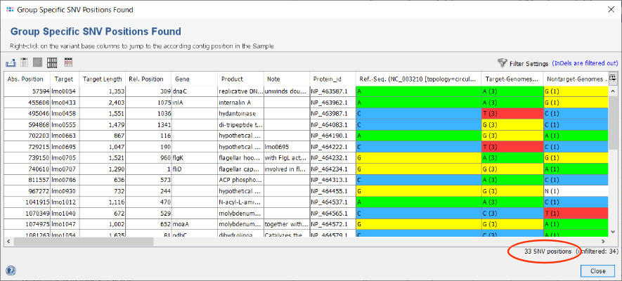
- Step 4: The found SNVs can be filtered further on by pressing the button
 in the upper right corner of the window. For example, choose in the upcoming filter dialog the option Show only SNV positions that change the GC content. Press the OK button to confirm this selection and apply the filtering. The table is now reduced to the 31 SNVs that passed the filter settings. Such a filter is beneficial if the intention is to design a high-resolution melting curve (HRMC) assay.
- Step 5: The Export button can be used to export the shown SNVs to a table file (CSV/XLSX). Furthermore, by selecting a SNV row and then right-clicking the target sequence can be exported. Both files are useful when using a primer design tool (e.g., ABI Primer Express tool) for setting up a HRMC or TaqMan™ realtime PCR assay.
FOR RESEARCH USE ONLY. NOT FOR USE IN CLINICAL DIAGNOSTIC PROCEDURES.